Data checked 5 November 2026. Historical analysis, with each series ending at its latest available observation.
Why do home loan rates rise? Why do property prices sometimes keep climbing even when borrowing becomes expensive? And why can interest rates fall while buyers remain nervous?
Looking at interest rates alone gives us only part of the story. Put mortgage rates, inflation, property growth and unemployment on one chart, and a more useful picture emerges. These forces interact—but they do not move together neatly, and they cannot tell us exactly when to buy.
Core Finding: Across 194 overlapping quarters since 1978, the statistical correlation between mortgage rate levels and annual residential property growth is only +0.11—demonstrating that lower interest rates alone do not guarantee property price growth. Incomes, employment confidence, credit policies, and available housing supply fundamentally determine the outcome.
#Nearly seven decades in one chart
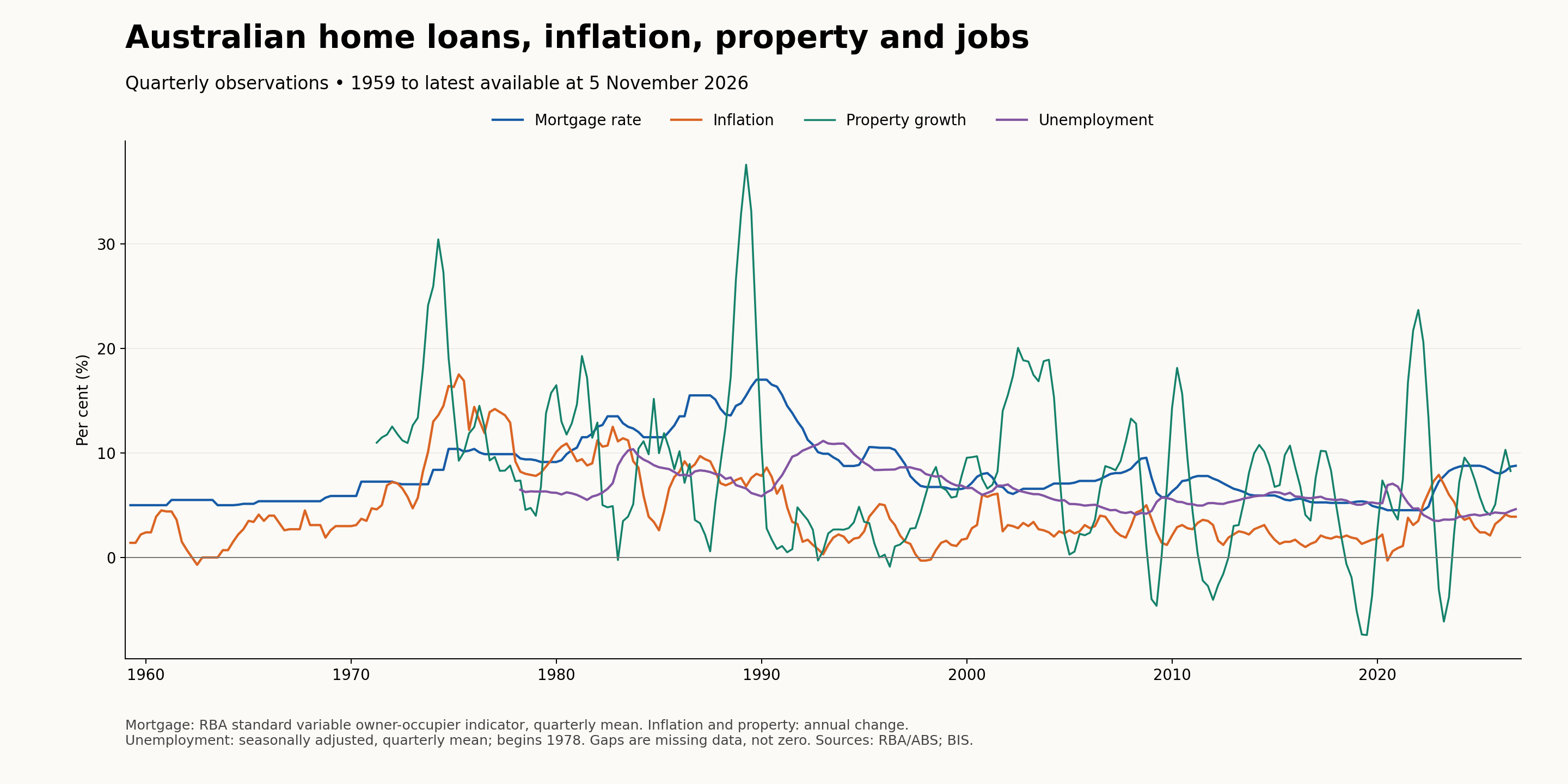
The chart begins in January 1959, the beginning of the selected RBA mortgage series. This is the beginning of this dataset, not the beginning of home lending in Australia. It includes every available quarter from then onward. Property growth begins in March 1971; the selected unemployment series begins in 1978. Missing years are left blank.
There is no single Australian home loan interest rate. Banks offer different fixed, variable, investor and owner-occupier rates. To tell a consistent historical story, this chart uses the RBA's standard variable owner-occupier housing loan indicator. It is an advertised benchmark, not the average rate borrowers actually pay. Discounts can make actual rates substantially lower. It is also different from the RBA cash rate.
#What the four lines mean
| Line | Plain-English meaning | Measurement |
|---|---|---|
| Mortgage rate | The annual interest rate on the selected benchmark home loan | Average of monthly observations within each quarter |
| Inflation | How quickly the general price of consumer goods and services increased | Headline CPI change from the same quarter a year earlier |
| Property growth | How quickly the selected Australian residential price measure increased or decreased | Nominal price change from the same quarter a year earlier |
| Unemployment | The share of people in the labour force who were unemployed | Average of monthly seasonally adjusted rates within each quarter |
All four use percentages, so they fit on one scale. But they measure different things. Mortgage rates and unemployment are levels; inflation and property growth measure annual changes. A crossing of two lines has no special economic meaning.
If property growth falls from 15% to 5%, prices are still rising, just more slowly. Prices fall year-on-year only when that line moves below zero. Likewise, falling inflation usually means prices are rising more slowly, rather than becoming cheaper.
The property series is a long historical composite. Its sources, geographic coverage and property mix change over time. Earlier observations include capital-city measures and detached houses; it should not be read as an identical nationwide all-dwelling sample throughout. It also does not describe every suburb.
#What is the latest picture in this chart?
| Indicator | Latest plotted observation | Reference period |
|---|---|---|
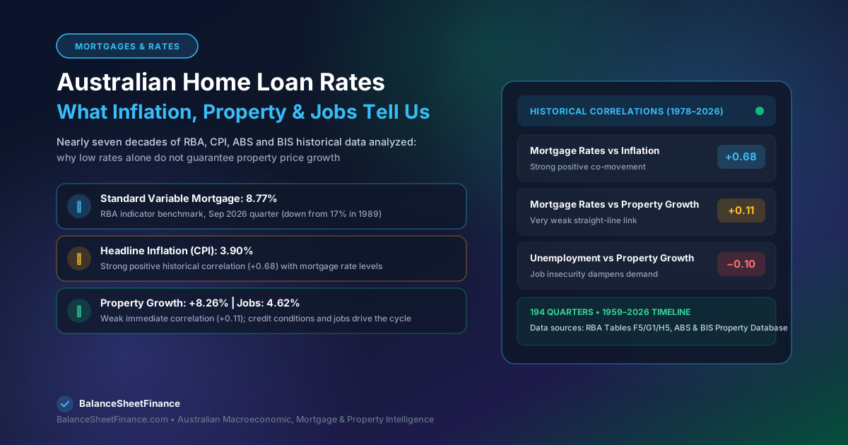
| Standard variable mortgage benchmark | 8.77% | September quarter 2026 average |
| Headline inflation | 3.90% | September quarter 2026 annual change |
| Residential property growth | 8.26% | June quarter 2026 annual change |
| Unemployment | 4.62% | September quarter 2026 average |
These observations have different dates. Property data is released with a delay. The chart therefore does not claim to show property growth through November 2026. The mortgage figure is a historical benchmark, not a quote for a loan you could obtain today.
#Pattern one: inflation and mortgage rates have a strong historical connection
Inflation reduces what money can buy. If groceries that cost $100 rise to $105, that basket has become 5% more expensive.
When inflation is persistent, the RBA can raise its cash-rate target to restrain spending and demand. Bank lending rates generally respond, though not always immediately or by exactly the same amount. Higher repayments leave borrowers with less money to spend. Businesses also face higher financing costs. Over time, this can reduce price pressure.
The chart shows high inflation and high mortgage rates during parts of the 1970s and 1980s. The underlying monthly standard variable mortgage series reached 17% in 1989.
But high rates appearing alongside high inflation does not mean high rates caused that inflation. Often, rates were raised in response to inflation already being high. The order of events matters.
#Pattern two: lower rates can help property prices—but do not guarantee growth
A lower rate reduces repayments on a given loan. It can also increase how much some buyers can borrow, increasing competition for homes.
For an illustration, a $700,000 principal-and-interest mortgage over 30 years costs approximately:
| Illustrative interest rate | Monthly repayment | 30-Year Total Repayments |
|---|---|---|
| 5.00% | $3,758 | $1,352,761 |
| 6.00% | $4,197 | $1,510,887 |
| 7.00% | $4,657 | $1,676,575 |
Repayment Buffer: Moving from 5% to 7% adds about $899 a month ($10,788 per year). A lower repayment does not automatically mean a buyer will qualify for a larger loan: Australian lenders assess income, living expenses, other debts, and a mandatory 3.00% serviceability buffer.
The chart shows strong property growth during the low-rate pandemic period. It also shows periods when property growth slowed or turned negative despite relatively low mortgage rates. Population, available homes, credit conditions, incomes, investor demand and expectations can all affect the outcome.
#Pattern three: job security changes how people respond to cheaper loans
Imagine two households offered the same rate reduction.
One has secure employment and enough savings. It may feel comfortable buying. The other fears losing an income. It may delay the purchase even though the loan has become cheaper.
This explains why falling rates are not automatically a sign that the economy or property market is healthy. Rates may be falling because conditions are weakening. Rising unemployment can reduce confidence and borrowing capacity and increase repayment stress.
The chart also shows why a simple rule is unreliable: the timing and strength of the unemployment–property relationship vary across episodes.
#Which combinations matter?
The following are economic interpretations, not rules proven by the chart or price forecasts.
| Combination | What it may mean | What a homeowner should examine |
|---|---|---|
| Inflation easing, rates falling, unemployment stable | Borrowing conditions may improve without a major deterioration in jobs | Whether local buyer competition is increasing |
| Inflation high, rates rising, unemployment low | Borrowers face pressure, while employment may still support demand | Repayments and the household cash buffer |
| Rates falling, unemployment rising | Cheaper credit may be offset by weaker confidence and income security | Whether the household could cope with losing an income |
| Rates high, property growth positive | Other sources of demand or limited supply may be supporting prices | Comparable sales rather than assuming high rates guarantee discounts |
| Property growth negative, employment stable | Some buyers may gain negotiating room, but local conditions vary | Whether suitable homes are actually cheaper and affordable |
For example, a rate cut accompanied by secure employment can have a different effect from a rate cut during a downturn. The reason for the cut matters as much as the cut itself.
#What happens when we calculate the relationships?
To go beyond eyeballing the chart, we calculated Pearson correlations using the 194 complete overlapping quarters from March 1978 to June 2026.
Correlation measures how closely two series move together. It ranges from −1 to +1. Values near zero indicate little straight-line association; positive values indicate movement in the same direction. It does not establish cause and effect.
| Pair, measured in the same quarter | Correlation | Interpretation for this sample |
|---|---|---|
| Mortgage-rate level and inflation | +0.68 | A relatively strong positive association |
| Mortgage-rate level and property growth | +0.11 | A weak positive association |
| Unemployment and property growth | −0.10 | A weak negative association |
The second result is particularly useful. The full history does not support a strong, simple relationship where a lower mortgage-rate level always coincides with faster property growth.
That does not mean rates have no effect. Rates respond to economic conditions; property responds to several forces; and both relationships can change over time. The analysis also mixes different economic regimes and a property series with historical coverage changes.
As an additional check, the correlation between today's mortgage-rate level and property growth four quarters later was only about +0.05 in the overlapping sample. This is not a causal estimate, a test of unexpected rate changes, or a forecasting model. A proper investigation would examine rate changes, multiple delays, different time periods and other influences together, and test forecasts on unseen data.
#Timing matters: the economy does not respond overnight
A rate change can affect market expectations quickly, while household spending and inflation take longer to adjust. Fixed-rate borrowers may not feel a change until their fixed term ends. Sellers may take time to accept lower offers. Businesses can delay hiring or investment decisions.
The RBA describes monetary policy as operating with long and variable delays. There is no fixed number of months after which a hike or cut guarantees a property-price response.
This is why a chart is best used to understand the economic setting, rather than to search for a perfect intersection that announces “buy now”.
#What does this mean for someone upgrading their home?
Suppose you own a home in Clyde North and want to move to Oakleigh. National interest rates matter, but the price difference between your current home and the home you want matters too.
Consider these purely illustrative numbers:
| Scenario | Current home | Target home | Price gap before costs |
|---|---|---|---|
| Before a fall | $800,000 | $1,400,000 | $600,000 |
| Both fall 5% | $760,000 | $1,330,000 | $570,000 |
The Upgrade Calculation: In this example, the price gap narrows by $30,000, even though the nominal value of the existing home falls. However, higher mortgage repayments or transaction costs (stamp duty, agent fees) could offset that benefit.
For a near-new home with at least four bedrooms, three bathrooms and a double garage, check sales of homes with those features. A national price index or a suburb median may tell a different story from that particular segment.
Before upgrading, compare your realistic sale proceeds after repaying the existing loan, the full purchase and selling costs, the new repayment, and your ability to manage a rate increase or temporary income loss. Those numbers turn the economic story into a household decision.
#The practical lesson
The four lines reveal an economy with feedback loops:
- Inflation influences rate decisions.
- Rates influence spending, borrowing capacity, and servicing stress.
- Employment influences buyer confidence and repayment capacity.
- Property prices respond to all of those forces, alongside local supply constraints and housing demographics.
The most useful question is therefore: What combination are we facing, and can our household afford the move under less favourable conditions?
History can help us ask better questions. It cannot promise the next direction of home loan rates or property prices.
#Sources and calculation notes
- RBA statistical tables: F5, G1 and H5. Direct downloads: F5, G1, H5. Series FILRHLBVS and GCPIAGYP; H5 seasonally adjusted unemployment rate. RBA/ABS and the underlying sources identified in those tables.
- BIS Australian nominal residential property price growth, Q.AU.N.771. Sources: national sources and BIS Residential Property Price database. Data downloaded from the selected property prices bulk file.
- BIS selected property price documentation and historical long-series documentation explain compilation and coverage differences.
- RBA: The Transmission of Monetary Policy explains the channels and delays.
- RBA: Monetary Policy Transmission through the Lens of the RBA's Models discusses model-based analysis and long, variable delays.
Quarterly mortgage and unemployment values are arithmetic means of available monthly observations. CPI and BIS growth retain their published quarterly annual-change values. No missing values were filled. Correlations use unrounded observations. The four-quarter check pairs each complete quarter's mortgage rate with property growth four quarters later. Data may be revised. Supporting observations are in australian-rates-and-property-data.csv.
General educational information; examples are not a recommendation to buy, sell or choose a particular loan.